
In this note we explore the possibilities to use these differences in order to obtain a better fitting result. We can express the qualities as either importance weights attached to the data points, or as a scale factor in the residuals.
Mostly data points are measured at locations (in time, space, frequency etc.) that are known with much higher precision than what is measured. These locations are called the independent variables, and what is measured at these locations, are called the dependent variables. In these cases, we fit the model by minimizing the mismatches in the dependent variable, called y, assuming that the other variable, the independent one, called x, is known with a precision, at least an order of magnitude better.
Assume we have N data points D = {xi,yi}. We want to fit the data with an as-yet-unspecified model
such that some norm of the residuals, ri, are minimumized over the parameters, θ.

The common suggestion, repeated in our paper, that the choice between weights and scales is irrelevant with respect to the final fitting results, is somewhat too fast. Up on closer inspection it turns out that the least-squares results and the maximum likelihood results are indeed the same, provided that we choose w = σ-2, where w is the weight and σ is the accuracy. However, the calculation of the size of the posterior and consequently, the evidence is different. The overall shape of the posterior is not affected.
The crux is in the likelihood. The likelihood is the product of the error distribution values at individual data points, xi.

When we choose a Gaussian error distribution we obtain for individual data points, without weights. We will address other error distributions later on in this note.

where yi is the measured value at location xi and mi = F(xi : θ). It is the value returned by the model, F, at the same location and for certain values of the parameter vector, θ, also known as mock data.. The scale factor, σ, is in the narrative of KM, part of the likelihood. It is either a fixed value or a hyperparameter to be estimated in the problem too.
The likelihood of Eq. 2 is displayed in Fig. 1, using the black line. It is shown as a function of the residuals r = y - m. The scale factor σ, is set to 1.0.

| Figure 1. The Gaussian likelihood as function of residual size. In black for σ = 1, in green for w = 2, and in red for σ = ½√2. |
When there are qualitative differences between individual data points, there are 2 ways to handle them: via weighting of the datapoints, and via scaling of the residuals. For weighting we assume that a data point that has a weight, w has the same impact as w (of the same) data points with a weight equal to 1. We can easily extend this to floating values of the weight, wi.
With these assumptions Eq. 4 transforms into

This is the formula we have been using in our NestedSampler.
In Fig. 1 the likelihood of Eq. 5 is displayed in green for a weight value, w = 2. This likelihood is not normalized as it is actually a product of 2 likelihoods of the form of Eq. 4. The latter is less than 1, everywhere, so the green line is consistently below the black line.
However, there is another option, where we know the accuracy of the errors on the data point, e.g. when the data point is the result of a previous calculation. Assume σi represents the size of the errors. In this narrative the σ's are a given. They are part of the data, not part of the likelihood.

The likelihood of Eq. 6 is shown in Fig.1 as the red line, using a value for σ = 1/ √2. This is a normalized likelihood, so when the width decreases, the height must increase.
Even if we put, as usual w = s-2 (as in Fig.1), there is still a difference between Eq. 5 and Eq. 6. The exponential parts of the equations turn out the same, but the normalizing parts are different. The least-squares and the maximum likelihood solutions only depend on the exponential parts. So they do not differ in both representations of the data quality. The Bayesian solution, posterior and evidence, take the full likelihood into account, so they are different. Which one is better is up to the user to decide: which of the notions, weighting or scaling, reflects better on the problem and the data at hand.
In the logarithm the likelihood transform into

Eq. 4 (no differing data quality) transforms (N is the number of data points).

Equation 5 (using weights) transforms into.

Equation 6 (using scales) transforms into.

There are several narratives that can be followed, each valid in applicable circumstances. Here we assume that the likelihood is a Gaussian error distribution.

The scale, σ, is either a given of the problem or an extra (hyper)parameter, that must be estimated from the data.

Errors in the model can occur simultaneously to errors in the data points. When combining 2 possible errors, the distribution takes the form of a convolution of both individual error distributions. For Gaussian distributions we obtain another Gaussian where the variance is the sum of the individual variances. For other distributions it is not so clear cut. In section 4 we discuss that situation.

All σ values might be the same for all data points, provided they are a given in the problem. Only one of them can be sensibly estimated from the data.

And in addition to Eq. 2 we have an extra residual to minimize; this time for the unknown x-location, for which holds that

The unknown x-locations are so called nuisance parameters of the problem, each with their own prior. They have to be integrated over all possible values to obtain the values for the model parameters, θ. When using the nested sampling algorithm, it means that the nuisance parameters just can be ignored.
PG1 presents a case where the nuisance parameters are integrated analytically, so they are removed from the problem. PG1 needs to assume that the model is a straight line and that one prior suffices for all targets. The latter encodes the case where the possible range of the values for the targets, t, is much smaller than the possible range of the errors, εi. PG1 ends up with one (maybe 2) nuisance parameters in stead of N.
We think that these conditions are too restrictive; we prefer working with nuisance parameters for the N targets. Again. using a Gaussian error distribution, we multiply the probabilities of Eqs. 11, 12, or 13, whatever the case is, with the probability for the residuals in x.

where τ is the accuracy of the data points in the x-direction.
As the targets are (nuisance) parameters to the problem, they need a prior. As said before, PG1 chooses a single prior for all targets and he could integrate the nuisance parameters out (for straight line models). We want a prior for each target as we think that in most cases the values for xi are not drawn from a single distribution, but are significantly different in themselves with an added error contribution. This leads to priors which are centered on the data point values of xi. This may seem like cheating as we are using the data for establishing the prior. But it is not. We know beforehand that the targets need to be near the x-data, whatever these data points are. We are not looking at the data and decide what to choose; we already know what to do.
Moreover, for a large class of distributions that are function of the size of the mismatch between target and data, it holds that the probability of the data, given the target, is the same as the probabilty of the target given the data. E.g. for a Gaussian distribution as prior
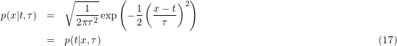
where the scale of the distribution, τ, needs to be specified, estimated by the user.
In its simplest form the likelihood becomes

The values of mi are now evalutated on the targets of x: mi = F(ti : θ).
More succinctly, the likelihood can be written in matrix notation as

where

So zi is the data vector, the ζi is the target vector and Vi is the variance matrix. The variance matrix contains σy being the accuracy deemed for the y-data, eventually compounded by the accuracy (known or unknown) for the model values at the target values, t, as in Eq. 5. The values for σx are the accuracies deemed for the x-data. Both σ's might be known on the level of individual data points, or only globally for the problem as a whole.
When there are errors on both axes, the contours of equal likelihood form nested ellipsoids, whose semimajor axes are multiples of σx and σy. The target positions, t, are found where these ellipisoids touch the model function, F. The optimal solution is found where the distances from data to targets is minimal. Geometrically, we have to find those parameters, θ, for which the ellipsoidal distance from data to model is minimal.

where ρi is the covariance factor between xi and yi. With this replacement, the likelihood of Eq. 18 stays the same.
With correlated errors, the ellipsoids are rotated according to the correlation between x and y. We still want to find the minimum in the ellipsoidal distances from data to model.
By construction the the errors in the differences are (anti)correlated. Every error in B shows negative in U - B and positive in B - V.
If the accuracies of U, B and V were σU, σB, and σV, resp., the covariance matrix would be

All this, of course, under conditions of independent measurements

The model mismatch is supposed to be independent of the other accuracies; it does not affect the covariance.

Where the v's are (co)variances of y and x.
The determinant of V becomes

And the inverse of V is

In most computations we need the likelihood in logarithmic form.

All relevant items in Eq. 28 need indices i. They are omitted to keep it (relatively) simple.
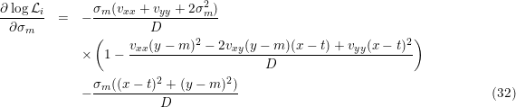
We also need the partial derivatives of the log-likelihood to the parameters, θ, to the targets, t, and, if present to the unknown model accuracy, σm as in Eq. 23.


Where δi,k is the Kronecker delta.
The unknown model scale is present in vyy, vxx, and subsequently in D.

So in case of Eq. 23 we have

Combining these
In the table below is indicated what is implemented in BayesicFitting with ✓, and what is not implemented with ✗. The numbers in brackets refer to notes.
The orange σm indicate a scale factor due to the incompleteness of the model. It might either be known or unknown. In the latter case the scale needs to be estimated from the data. All other scales are known accuracies that need to be presented with the data.
| ErrorDistributions | |||||||
|---|---|---|---|---|---|---|---|
| Scale | Eqn | Gauss | Laplace | Uniform | Expon | Cauchy | Mixed |
| σ | 11 | ✓ | ✓ | ✓ | ✓ | ✓ | ✗ (1) |
| σm | 11 | ✓ | ✓ | ✓ | ✓ | ✓ | ✓ |
| σi | 12 | ✓ | ✓ | ✓ | ✓ | ✓ | ✗ (1) |
| σi + σm | 13 | ✓ | ✗ (2) | ✗ (3) | ✗ (2) | ✗ (2) | ✗ (4) |
| Errors in X and Y (5) | |||||||
| ( σi, τi ) | 18 | ✓ | ✓ (6) | ✓ (6) | ✓ (6) | ✓ (6) | ✗ (1) |
| ( σi, τi, ρi ) | 21 | ✓ | ✗ (7) | ✗ (7) | ✗ (7) | ✗ (7) | ✗ (1) |
| ( σi + σm, τi + σm, ρi ) | 22 | ✓ | ✗ (2) | ✗ (3) | ✗ (2) | ✗ (2) | ✗ (4) |
| Notes | |||||||
| 1 | Only of interest when both scales of the mixing distributions are unknown. | ||||||
| 2 | Convolution distribution unknown | ||||||
| 3 | Convolution is a chopped triangular distribution. | ||||||
| 4 | Only when both mixed distributions are Gauss. | ||||||
| 5 | Assuming the same distribution in X and Y. | ||||||
| 6 | Could in principle be done. However not implemented yet for want of a good use case. | ||||||
| 7 | Dont know; Maybe a rotated version of the previous. Analogous to Gauss. | ||||||
The overall likelihood is the product of the likelihoods of the individual points, as in Eq. 3. Using weights Eq. 3 changes in

It is irrelevant what the exact form of the individual likelihoods is.
They can all be combined in this way with weights.