83 Aquarii
83 Aqr is a visible double star with a period of about 20 years and aseparation of 0.2 arcsec.
We have data from SIDONIE (https://sidonie.oca.eu) and WDS
(https://www.usno.navy.mil/USNO/astrometry/optical-IR-prod/wds/int4)
Author: Do Kester
We need to import some classes
In[1]:
import numpy as numpy
import math

from astropy.io import ascii
from BayesicFitting import StellarOrbitModel
from BayesicFitting import MultipleOutputProblem
from BayesicFitting import PolynomialModel
from BayesicFitting import CircularUniformPrior

from BayesicFitting import NestedSampler
from BayesicFitting import formatter as fmt
from BayesicFitting import plotFit
from BayesicFitting import Tools
import matplotlib.pyplot as plt
In[2]:
#%matplotlib osx
Read the data
In[3]:
tbl = ascii.read( "/Users/do/Projects/DoubleStars/83Aqr/83Aqr.dat", include_names=['Date', 'Angle',
                                'Separ', 'err-a', 'err-s', 'nts', 'pr'] )
# print( tbl )
# The table lists:
#   fractional years
#   angle in degree
#   separation in arcsec
#   number of nights the star is observed
#   precision in number of decimals in the separation (2 or 3)
yr0 = tbl['Date'].data
phi = tbl['Angle'].data
dis = tbl['Separ'].data
erp = tbl['err-a']
erd = tbl['err-s']
nts = tbl['nts'].data
prc = tbl['pr'].data

#phi = numpy.where( phi > 300, phi - 360, phi )
In[4]:
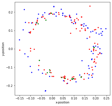
th = phi * math.pi / 180

## Do we need a correction for leap years. They are 0.3% longer
yr1 = yr0 - 1900
#xpos = dis * numpy.cos( th )
#ypos = dis * numpy.sin( th )
xpos = dis * numpy.sin( th )
ypos =-dis * numpy.cos( th )

plt.figure( "data", figsize=(6,6) )
q = numpy.where( yr0 <= 1900 )
plt.plot( xpos[q], ypos[q], 'k.' )
q = numpy.where( numpy.logical_and( 1900 <= yr0, yr0 < 1950 ) )
plt.plot( xpos[q], ypos[q], 'b.' )
q = numpy.where( numpy.logical_and( 1950 <= yr0, yr0 < 2000 ) )
plt.plot( xpos[q], ypos[q], 'r.' )
q = numpy.where( yr0 >= 2000 )
plt.plot( xpos[q], ypos[q], 'g.' )
plt.xlabel( 'x-position' )
plt.ylabel( 'y-position' )
plt.show()
Out[4]:
A bit of data massaging.
In[5]:
## Do we need a correction for leap years. They are 0.3% longer
yr = yr0 - 1900

# Make weights proportional to the number of nights observed and
# divide by 4 if the precision is given in 2 decimals in stead of 3
#wgt = numpy.where( prc == 3, nts, nts / 4 )
#wgt = numpy.sqrt( nts ) * numpy.power( 10.0, prc - 3 )
erd = numpy.where( erd == 0, 100, erd )
#wgt = nts / ( numpy.square( 100 * erd ))
rwgt = nts / ( 100 * erd )
rwgt = numpy.where( rwgt > 30, 30.0, rwgt )
rwgt = numpy.where( prc == 0, 0.0, rwgt )

erc = numpy.array( [100, 10, 5, 2, 1], dtype=float )
erp = numpy.where( erp == 0, erc[prc], erp )
pwgt = nts / erp
pwgt = numpy.where( prc == 0, 0.0, pwgt )

pwgt *= 0.1                ## to balance with rwgt

d2r = math.pi / 180

pwgt *= d2r

# Combine xpos and ypos into a 2-d array: pos
pos = numpy.append( dis, th ).reshape( 2, -1 ).transpose()
wgt = numpy.append( rwgt, pwgt ).reshape( 2, -1 ).transpose()
We define a stellar orbit model. It has 7 parameters: eccentricity,
semimajor axis, period, periastron phase, inclination of the orbit,
longitude of ascending node and phase of the ascending node.
All 4 phase parameters get a CircularUniformPrior 0 to 2 pi.
In[6]:
twopi = 2 * math.pi
mdl = StellarOrbitModel( spherical=True )
## eccen, semimaj, period, phase, inclin, node phase, node pos
lolim = [0.0, 0.0, 20.0]
hilim = [0.9, 1.0, 30.0]
mdl.setLimits( lowLimits=lolim, highLimits=hilim )
#Tools.printclass( mdl )

mdl.setPrior( 3, prior=CircularUniformPrior(), limits=[0,twopi] )       ## phase of periastron
mdl.setPrior( 4, prior=CircularUniformPrior(), limits=[0,math.pi] )     ## inclination
mdl.setPrior( 5, prior=CircularUniformPrior(), limits=[0,math.pi] )     ## from North to line of nodes
mdl.setPrior( 6, prior=CircularUniformPrior(), limits=[0,twopi] )       ## fron line of nodes to periastron
#Tools.printclass( mdl )
Define a MultipleOutputProblem which reorganises the multiple outputs:
(x,y) into a 1-d array that can be handled by the NestedSampler.
Define NestedSampler with extended ensemble for better precision.
In[7]:
problem = MultipleOutputProblem( model=mdl, xdata=yr, ydata=pos,
                                weights=wgt )
# define NestedSampler
ns = NestedSampler( problem=problem, seed=80409 )
ns.ensemble = 500

#ns.engines[0].verbose = 5

# set limits on the noise scale of the distribution
ns.distribution.setLimits( [0.01,100] )
# ns.verbose = 2
# run NestedSampler
evi = ns.sample( )
Out[7]:
Fit all parameters of
  StellarOrbit
Using a Gauss error distribution with with unknown scale
Moving the walkers with   GalileanEngine  ChordEngine
>>>>>>>>>>>>>>>>>>>>>>>>>>>>>>>>>>>>>>>>>>>>>>>>>>
>>>>>>>>>>>>>>>>>>>>>>>>>>>>>>>>>>>>>>>>>>>>>>>>>>
>>>>>>>>>>>>>>>>>>>>>>>>>>>>>>>>>>>>>>>>>>>>>>>>>>
>>>>>>>>>>>>>>>>>>>>>>>>>>>>>>>>>>>>>>>>>>>>>>>>>>
>>>>>>>>>>>>>>>>>>>>>>>>>>>>>>>>>>>>>>>>>>>>>>>>>>
>>>>>>>>>>>>>>>>>>>>>>>>>>>>>>>>>>>>>>>>>>>>>>>>>>
>>>>>>>>>>>>>>>>>>>>>>>>>>>>>>>>>>>>>>>>>>>>>>>>>>
>>>>>>>>>>>>>>>>>>>>>>>>>>>>>>>
Iteration   logZ        H     LowL     npar    parameters
   38002   1.48e+03     38.0   1.52e+03      8  [    0.357    0.202   21.810    5.117    0.798    0.454    4.600    0.010]
Engines              success     reject     failed       best      calls
GalileanEngine        265627      81206      91904         39      38051
ChordEngine           266230     446883          0         53      38051
Calls to LogL        1151850   to dLogL      81206
Samples       38502
Evidence       640.648 +-      0.120
In[ ]:
Print parameters and standard deviations, first as they were derived and
then in an alternative form with angles in ``degrees'' and the
periastron in years.
In[8]:
sl = ns.samples
par = sl.parameters
std = sl.stdevs
pard = par.copy()
pard[3:] *= 180 / math.pi
pard[3] *= pard[2] / 360
pard[3] += 1900
stda = std.copy()
stda[3:] *= 180 / math.pi
stda[3] *= pard[2] / 360
names = mdl.parNames
print( "         ", end="" )
for nm in names :
    print( " %8.8s"% nm, end="" )
print()
print( "Pars   ", fmt( par, max=None ) )
print( "Stdev  ", fmt( std, max=None ) )
print( "Par_alt", fmt( pard, max=None ) )
print( "Std_alt", fmt( stda, max=None ) )
print( "Scale     ", fmt( sl.scale ), "+-", fmt( sl.stdevScale ) )
print( "Evidence  ", fmt( evi ) )
print( "periastron times" )
for k in range( -3, 6 ) :
    print( fmt( pard[3] + k * par[2] ), end='' )
print()
Out[8]:
          eccentri semimajo   period phase si inclinat north2no nodes2pe
Pars    [    0.357    0.202   21.811    5.115    0.799    0.452    4.600]
Stdev   [    0.012    0.001    0.030    0.035    0.011    0.027    0.016]
Par_alt [    0.357    0.202   21.811 1917.757   45.769   25.909  263.585]
Std_alt [    0.012    0.001    0.030    0.122    0.647    1.568    0.909]
Scale          0.010 +-     0.000
Evidence     640.648
periastron times
 1852.325 1874.136 1895.946 1917.757 1939.567 1961.378 1983.189 2004.999 2026.810
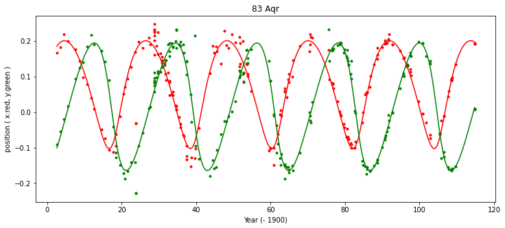
In[9]:
plt.figure( "results", figsize=(12,5) )
plt.plot( yr, xpos, 'r.' )
plt.plot( yr, ypos, 'g.' )
xx = numpy.linspace( yr[0], yr[-1], 201, dtype=float )
rp = mdl.result( xx, par )

xpf = rp[:,0] * numpy.sin( rp[:,1] )
ypf =-rp[:,0] * numpy.cos( rp[:,1] )


plt.plot( xx, xpf, 'r-' )
plt.plot( xx, ypf, 'g-' )

plt.xlabel( "Year (- 1900)")
plt.ylabel( "position ( x:red, y:green )")
plt.title( "83 Aqr" )
plt.show()
Out[9]:
In[10]:
plt.figure( "orbit", figsize=(6,6) )

mkrp = mdl.result( yr, par )

xmk = mkrp[:,0] * numpy.sin( mkrp[:,1] )
ymk =-mkrp[:,0] * numpy.cos( mkrp[:,1] )

q = numpy.where( yr0 <= 1900 )
plt.plot( xpos[q], ypos[q], 'k.' )
for k in q :
    plt.plot( [xmk[k],xpos[k]], [ymk[k],ypos[k]], 'k-' )

q = numpy.where( numpy.logical_and( 1900 <= yr0, yr0 < 1950 ) )
plt.plot( xpos[q], ypos[q], 'b.' )
for k in q :
    plt.plot( [xmk[k],xpos[k]], [ymk[k],ypos[k]], 'b-' )

q = numpy.where( numpy.logical_and( 1950 <= yr0, yr0 < 2000 ) )
#q = numpy.where( numpy.logical_and( 1990 <= yr0, yr0 < 2000 ) )
plt.plot( xpos[q], ypos[q], 'r.' )
for k in q :
    plt.plot( [xmk[k],xpos[k]], [ymk[k],ypos[k]], 'r-' )

q = numpy.where( yr0 >= 2000 )
plt.plot( xpos[q], ypos[q], 'g.' )
for k in q :
    plt.plot( [xmk[k],xpos[k]], [ymk[k],ypos[k]], 'g-' )

xx = numpy.linspace( yr[0], yr[-1], 201, dtype=float )
yy = mdl.result( xx, par )

xf = yy[:,0] * numpy.sin( yy[:,1] )
yf =-yy[:,0] * numpy.cos( yy[:,1] )

# plot the orbit
plt.plot( xf, yf, 'k-' )

#plot the center
plt.plot( [0.0], [0.0], 'k*' )

# plot line to periastron
yperi = mdl.result( [par[3] * par[2] / ( 2 * math.pi )], par )
xpr =  yperi[0,0] * math.sin( yperi[0,1] )
ypr = -yperi[0,0] * math.cos( yperi[0,1] )
plt.plot( [0.0,xpr], [0.0,ypr], 'k-')

# plot line of nodes
xas = 0.3 * math.sin( par[5] )
yas =-0.3 * math.cos( par[5] )

plt.plot( [-xas,xas], [-yas,yas], 'm-')
plt.plot( [xas], [yas], 'ms' )
plt.axis('equal' )
plt.show()
Out[10]:
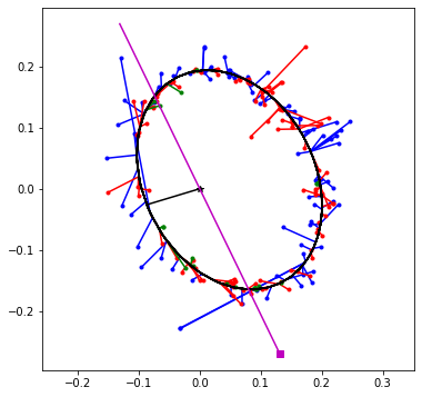
In the picture above we see the orbit of 83 Aqr as it appears on the
sky. (North down, east left TBC). The black ellipse is the projected
orbit of the secundary star. It is moving anti-clockwise. The
observations at the colored points are connected to the orbit location
at the same time. The colors indicate when they are taken: blue < 1950;
1950 < red < 2000 and green > 2000.
The main star is located at (0,0) where the back * is plotted. Through
it in magenta is the line of nodes, i.e. where the sky through the main
star crosses the orbit. The magenta square indicates where the ascending
node is located, the place where the orbiting star crosses the sky plane
and is moving toward us. At the other side, at the descending node, the
orbiting star crosses the sky plane away from us. The black line from
the main star to the orbit indicate the lacotion of the periastron, the
place where the stars as closest together. The periastron lies behind
the sky plane.
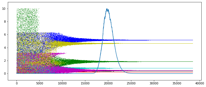
In[11]:
plt.figure( 2, figsize=[12,5] )
pev = sl.getParameterEvolution()
c = ['k,', 'r,', 'g,', 'b,', 'c,', 'm,', 'y,']
for k in range( mdl.npars ):
    if k == 2 :
        plt.plot( pev[:,k] - 20, c[k] )
    else :
        plt.plot( pev[:,k], c[k] )
wev = sl.getWeightEvolution()
wev /= numpy.max( wev )
plt.plot( wev * 10 )
plt.ylim( -1, 11 )
plt.show()