Radio Astronomy Spectrometer
Table 12.4 from Phil Gregory book is copied.NestedSampler is used to find the probability of a source present in the data.
Author: Do Kester
import stuff
In[1]:
import numpy as numpy
import math

from BayesicFitting import GaussModel
from BayesicFitting import PolynomialModel
from BayesicFitting import ConstantModel
from BayesicFitting import NestedSampler
from BayesicFitting import formatter as fmt
from BayesicFitting import plotFit
import matplotlib.pyplot as plt
In[2]:
x = [k for k in range(1,65)]
y = [0.82,-2.07,0.38,0.99,-0.12,-1.35,-0.20, 0.36,-.78,1.01,
     0.44,0.34,1.58,0.08,0.38,-0.71,-0.90,0.33,0.80,-1.42,
     0.28,-0.42,0.12,0.14,-0.63,-1.77,-0.67,0.55,1.98,-0.08,
     1.16,0.48,-0.03,1.47,1.70,1.89,4.55,3.59,2.02,0.21,
     0.05,0.54,-0.09,-0.61,2.49,0.07,-1.45,0.56,-0.72,0.38,
     0.02,-1.26,1.35,-0.04,-1.45,1.48,-1.16,-0.40,0.01,0.29,
     -1.35,-0.21,-1.67,0.70]
Define the model
In[3]:
mdl = GaussModel( )
print( mdl )
lo = [0,0,0]
hi = [10,64,10]
mdl.setLimits( lo, hi )
Out[3]:
Gauss: f( x:p ) = p_0 * exp( -0.5 * ( ( x - p_1 ) / p_2 )^2 )
define the fitter: Fitter
In[4]:
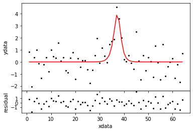
ns = NestedSampler( x, mdl, y )
ns.distribution.setLimits( [0.1, 10] )
evid = ns.sample( plot=True )
Out[4]:
Fit all parameters of
  Gauss: f( x:p ) = p_0 * exp( -0.5 * ( ( x - p_1 ) / p_2 )^2 )
Using a Gauss error distribution with with unknown scale
Moving the walkers with   GalileanEngine  ChordEngine
>>>>>>>>>>>>>>>>>>>>
Iteration   logZ        H     LowL     npar    parameters
    1971        -98      9.9      -85.5      4  [    3.922   37.210    1.590    0.900]
Engines              success     reject     failed       best      calls
GalileanEngine         13833       4545       2861         12       1971
ChordEngine            13766      14430          0          5       1971
Calls to LogL          49435   to dLogL       4545
Samples        2071
Evidence       -42.570 +-      0.136
In[5]:
sl = ns.samples
par = sl.parameters
In[6]:
print( "Parameters :", fmt( ns.parameters ) )
print( "StDevs     :", fmt( ns.stdevs ) )
print( "Scale      :", fmt( ns.scale ) )
print( "Evidence   :", fmt( evid ) )
Out[6]:
Parameters : [    4.100   37.177    1.638]
StDevs     : [    1.206    0.383    0.679]
Scale      :     0.963
Evidence   :   -42.570
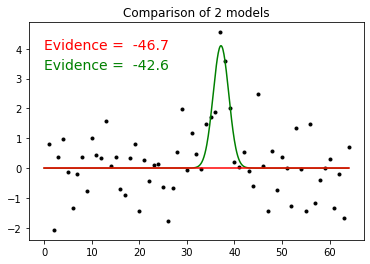
How probable is the existence of a source with these parameters. Compare
it with a fit of a constant model, which is always 0.
In[7]:
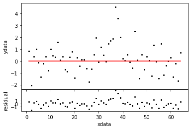
mdl0 = ConstantModel()
ns0 = NestedSampler( x, mdl0, y )
ns0.distribution.setLimits( [0.1,10] )
evid0 = ns0.sample( plot=True )
sl0 = ns0.samples
Out[7]:
Fit all parameters of
  ConstantModel: f( x ) = Polynomial: f( x:p ) = p_0
Using a Gauss error distribution with with unknown scale
Moving the walkers with   GalileanEngine  ChordEngine
>>>>>>
Iteration   logZ        H     LowL     npar    parameters
     553       -108      2.8       -104      1      1.236
Engines              success     reject     failed       best      calls
GalileanEngine          3851        480          2          3        553
ChordEngine             3942         97          0          1        553
Calls to LogL           8372   to dLogL        480
Samples         653
Evidence       -46.701 +-      0.072
The log(evidence) decreased by 3.9, meaning that the GaussModel is
10^3.9 = 8000 times more probable than the constant model
In[9]:
plt.figure( 1 )
plt.plot( x, y, 'k.' )
xx = numpy.linspace( 0, 64, 641 )
plt.plot( xx, mdl.result( xx, par ), 'g-' )
plt.plot( xx, mdl0.result( xx, [] ), 'r-' )

txt1 = "Evidence = %6.1f" % evid
txt0 = "Evidence = %6.1f" % evid0
plt.text( 0, 4, txt0, color='red', size=14 )
plt.text( 0, 3.3, txt1, color='green', size=14 )
plt.title( "Comparison of 2 models")
plt.show()

#plt.text( 13, 16.5, txt, size=14,
#         va="baseline", ha="left", multialignment="left",
#         bbox=dict(fc="none"))