Examples: HD76700

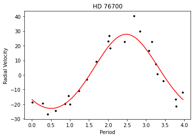
HD 76700

Radial velocity data for HD76700 were obtained from Tinney et al.(2003).
Author: Do Kester

We need to import some classes

In[1]:

import numpy as numpy
import math

from astropy.io import ascii
from BayesicFitting import RadialVelocityModel
from BayesicFitting import PolynomialModel
from BayesicFitting import CircularUniformPrior

from BayesicFitting import NestedSampler
from BayesicFitting import formatter as fmt
from BayesicFitting import plotFit
from BayesicFitting import Tools
import matplotlib.pyplot as plt

In[2]:

#%matplotlib osx

Read the data

In[3]:

tbl = ascii.read( "data/HD76700-Tinney.dat" )
#print( tbl )
jd = tbl['JDa'].data
rv = tbl['RVa'].data
er = tbl['Uncertainty'].data
wgt = 100.0 / numpy.square( er )

We define a radial velocity model. It has 5 parameters: eccentricity,
amplitude, period, phase of periastron, longitude of periastron. The
phase parameters both get a CircularUniformPrior. We need to add a
constant for the systemic velocity of the system.

In[4]:

twopi = 2 * math.pi
rvm = RadialVelocityModel( )
lolim = [0.0, 0.0, 3.0]
hilim = [0.9, 40.0, 5.0]
rvm.setLimits( lowLimits=lolim, highLimits=hilim )
rvm.setPrior( 3, prior=CircularUniformPrior(), limits=[0,twopi] )
rvm.setPrior( 4, prior=CircularUniformPrior(), limits=[0,twopi] )
#Tools.printclass( rvm )
pm = PolynomialModel( 0 )
pm.setLimits( lowLimits=[-20], highLimits=[20] )
#sm *= hm
mdl = pm + rvm
print( mdl )

Out[4]:

Polynomial: f( x:p ) = p_0 +
RadialVelocity

In[5]:

# define NestedSampler
ns = NestedSampler( jd, mdl, rv, weights=wgt, seed=1301 )
ns.ensemble = 500
# set limits on the noise scale of the distribution
ns.distribution.setLimits( [0.01,100] )

# run NestedSampler
evi = ns.sample( plot=True )

Out[5]:

Fit all parameters of
  Polynomial: f( x:p ) = p_0 +
  RadialVelocity 
Using a Gauss error distribution with with unknown scale
Moving the walkers with   GalileanEngine  ChordEngine
>>>>>>>>>>>>>>>>>>>>>>>>>>>>>>>>>>>>>>>>>>>>>>>>>>
>>>>>>>>>>>>>>>>>>>>>>>>>>>>>>>>>>>>>>>>>>>>>>>>>>
>>>>>>>>>>>>>>>>>>>>>>>>>>>>>>>>>>>>>>>>>>>>>>>>>>
>>>>>>>>>>>>>>>>>>>>>>>>>>>>>>>>>>>>>>>>>>>>>>>>>>
>>>>>>>>>>>>>>>>>>>>>>>>>>>>>>>>>>>>>>>>>>>>>>>>>>
>>>>>>>>>>>>>>>>>>>>>>>>>>>>>>
Iteration   logZ        H     LowL     npar    parameters
   27978       -353     28.0       -321      7  [    0.724    0.075   25.647    3.971    3.805    6.159    4.128]
Engines              success     reject     failed       best      calls
GalileanEngine        159283      56852      96987         58      30362
ChordEngine           212502    1126682          2         43      30362
Calls to LogL        1652308   to dLogL      56852
Samples       28478
Evidence      -153.510 +-      0.103

In[6]:

sl = ns.samples
par = sl.parameters
std = sl.stdevs
print( fmt( par, max=None ) )
print( fmt( std, max=None ) )
pal = par.copy()
stl = std.copy()
pal[5] *= 180 / math.pi
pal[4] *= 0.5 * pal[3] / math.pi
stl[5] *= 180 / math.pi
stl[4] *= 0.5 * pal[3] / math.pi
print( fmt( pal, max=None ) )
print( fmt( stl, max=None ) )
print( fmt( sl.scale ), fmt( sl.stdevScale ) )
print( evi )

Out[6]:

[    0.758    0.067   25.342    3.971    3.854    6.207]
[    0.528    0.026    0.755    0.000    0.492    0.493]
[    0.758    0.067   25.342    3.971    2.436  355.662]
[    0.528    0.026    0.755    0.000    0.311   28.219]
    4.268     0.339
-153.51027291941526

In[7]:

plt.plot( jd % par[3], rv, 'k. ' )
xx = numpy.linspace( 0, par[3], 1001, dtype=float )
plt.plot( xx, mdl.result( xx, par ), 'r-' )
plt.xlabel( "Period")
plt.ylabel( "Radial Velocity")
plt.title( "HD 76700" )
plt.show()

Out[7]:

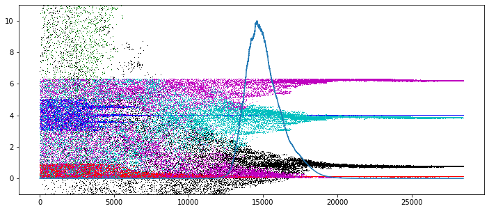
In[9]:

plt.figure( 2, figsize=[12,5] )
pev = sl.getParameterEvolution()
c = ['k,', 'r,', 'g,', 'b,', 'c,', 'm,']
for k in range( mdl.npars ):
    plt.plot( pev[:,k], c[k] )
wev = sl.getWeightEvolution()
wev /= numpy.max( wev )
plt.plot( wev * 10 )
plt.ylim( -1, 11 )
plt.show()

HD76700