
We have a paper out in "Astronomy and Computing" about BayesicFitting. Kester and Mueller (2021) or find it directly here.
It is assumed that the reader is familiar with the Bayesian ways to perform inference from data. If not, there are enough books on the market that explain what it is about. E.g. Sivia (2006), Bishop (2006), von der Linden (2014) and Jaynes (2003). The equations implemented in this toolbox can be found in Kester (2004).
The BayesicFitting toolbox can be used to fit data to a model and to find the model that fits the data best. The first goal is achieved by optimizing the parameters of the model in light of the data present. For the second goal the evidence is calculated, either as a Gaussian approximation, or in case of NestedSampler by integrating over the posterior.
The easiest way to get started with this package is to look into the examples directory and find an example that looks like the problem to be solved.
To run the examples start a notebook by typing
jupyter notebook
in the examples directory. Select the example in the list that appears in the browser. Copy and edit the example until it works on the problem at hand.
Glossary
A list of the terms used throughout this package, with explanations.
Troubles
A list of troublesome situations and what to do about it.
Design
An architectural design document, displaying the relationships between
the classes.
Style
A document about coding style adhered to by this project.
References
A list of external references for BayesisFitting.
The toolbox contains over 100 classes. Each class forms an object that encapsulates several methods. The name of the class is a good indication of the functionality of the object it generates. E.g. PolynomialModel generates a Model object that yields a polynomial of a selected order, etc. Similarly there are collections of Fitters, ErrorDistributions, Priors and Engines.
Each class and all of its methods are fully documented, using document strings.
The classes can be divided into 3 broad categories Models, Fitters and classes pertaining to the NestedSampler.
All classes must be imported with
from BayesicFitting import SomeClass
or of course with
from BayesicFitting import *
which imports all classes. In the remainder of this manual it is assumed that all necessary imports have been performed in the code listed.
A model is a class that encapsulates a relation between independent
variable, parameters and a dependent variable.
The independent variable is called x (or xdata); de parameters are
indicated as p (or pars, param or params) and the dependent
variable is called y (or ydata).
The relation between them is a mathematical function f.

The result of the function together with its derivatives, parameter values, and other possibly usefull information is packed into the class.
Assuming that m is a Model, all following attributes and methods are
defined.
np = m.nrpars                       # number of parameters in the model
p = m.parameters                    # list of parameters of the model
nd = m.ndim                         # number of dimensions in the model
r = m.result( xdata, pars )         # results of f(xdata:pars)
r = m( xdata )                      # short for m.result( xdata, p )
dfdp = m.partial( xdata, pars )     # partial derivative of f to p
dfdx = m.derivative( xdata, pars )  # derivative of f to x
name = m.__str__()                  # name of the model as a string
parname = m.parNames                # list of parameter names
Most Models are 1-dimensional i.e. they require a 1-dimensional input vector. Two- or more-dimensional models need 2 or more numbers for each result it produces. One could think of fitting maps or cubes. The results of any model is always a 1-dimensional vector, except when not.
In general, models of different dimensionality cannot be combined.
Simple models are objects that are created by invoking one model class.
m1 = PolynomialModel( 1 )
m2 = GaussModel()
Both m1 and m2 are simple models. The first assumes a linear relation
between xdata and ydata.

It has 2 parameters that can be optimized to fit the ydata.
The second model m2 encapsulates the function

It has 3 parameters to be fitted.
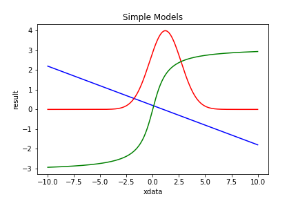
| Figure 1 shows 3 simple models: PolynomialModel (blue), GaussModel (red) and ArctanModel (green). |
A simple model is a Model, i.e. all actions valid for Models can be done with simple models.
Upon construction of a simple model the value(s) of one or more parameters can be fixed. Either with a constant value, turning the model into one with less parameters, or with another Model. In the latter case the parameter is changing as the Model. Results and derivatives are constructed from the interacting models.
A keyword argument, fixed=<dictionary>, is used to construct a fixed
model. The dictionary consist of an integer key, indicating the
parameter index, and a float value for fixing the parameter with a
constant, or a Model value for replacing the parameter by the model.
In the former case the fixed model has one parameter less than the original
model. In the latter case, the parameters of the replacing model are appended
to the parameters of the fixed model which also is one parameter less than
the original.
m1 = PolynomialModel( 1, fixed={0:0.0} )    # line through origin
m2 = GaussModel()
m3 = ArctanModel( fixed={0:m2} )        # Gauss-modulated arctangus
# Build a series of models of increasing polynomial order.
pm1 = PolynomialModel( 1 )                  # 1st order
pm2 = PolynomialModel( 1, fixed={1:pm1} )   # 2nd order
pm3 = PolynomialModel( 1, fixed={1:pm2} )   # 3rd order
# etc. But not as efficient as PolynomialModel( 3 )
See also the mrs-fringes example.
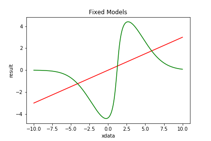
| Figure 2 shows the 2 fixed models listed above: PolynomialModel (red) and ArctanModel (green). |
Fixed models are non-linear, except when the model is linear and the parameters are fixed with constants.
A fixed model is a Model, i.e. all actions valid for Models can be done with fixed models.
Models can be combined by various operations (+, -, *, /, |) into a new (compound) model. The 4 arithmetic operators do the obvious: they take the results of both models and apply the operation. For compound models the (partial) derivatives, (parameter) names etc are properly defined.
All operations are also available as assignment operators: +=, -=, *=, /=, and |=.
To construct a gaussian emission line on a linearly changing background:
m4 = PolynomialModel( 1 ) + GaussModel()
To construct an absorption line with a voigt profile on a constant background:
m5 = PolynomialModel( 0 )
m5 -= VoigtModel()
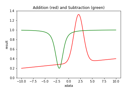
| Figure 3 shows examples of Compound Models using addition and subtraction. |
Using multiplication an alternative for m3 can be written as:
m6 = ArctanModel( fixed={0:1.0} ) * GaussModel()
Note that without the fixed keyword in ArctanModel, m6 would be
degenerate as both models have an amplitude parameter. By fixing one of
them to 1.0 the model avoids degeneracy.
To construct the inverse of (p0 + p1 * x2):
m7 = ConstantModel( values=1 ) / PolynomialModel( 2, fixed={1:0.0} )
The ConstantModel is a model without parameters that returns a constant value,
in this case 1.0 for any value of x.
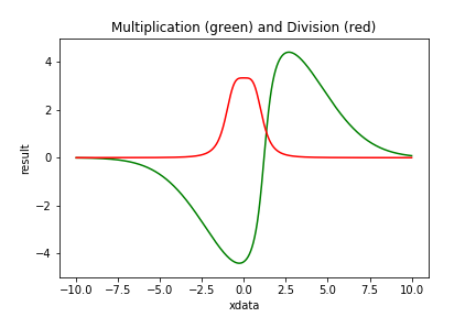
| Figure 4 shows examples of Compound Models using multiplication and division. |
A special operation that can be applied to two models is the pipe, indicated by |. It acts like the (unix) pipe: the result of the left-hand model is used as input of the right-hand model.
When m1, m2 and m3 are models implementing

then

The input of m2 is relacced by the result of m1. While in case of

the m1 only influences m2, not m3. To influence both m2 and m3, brackets are needed.

This is the only place where a 2-d model can be combined with a 1-d model as the output of a 2-d model is 1 dimensional. Or in general the output dimensionality of the left hand model must conform the input dimensionality of the right hand model.
In the FixedModels paragraph a gauss modulated arctan model was constructed. In that model the gauss and the arctan had its own x-shift parameter. Both parameters were set to the same value in Figure 2, making a balanced wave function.
To force them being the same, the x-shift parameters in both models are fixed to 0. Then x is shifted linearly and it is piped through the other models.
m10 = ArctanModel( fixed={0:1.0,1:0.0} ) * GaussModel( fixed={1:0.0} )
m11 = PolynomialModel( 1, fixed={1:1.0} ) | m10
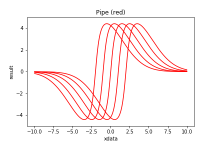
| Figure 5 shows examples of Compound Models with a pipe. |
Compound models are Models and can be combined with other (compound) models into a new model. This way quite complicated models can be formed without worrying about internal consistency. See the gaussfit example.
Compound models are non-linear unless all its constituents are linear and its operations are additive.
A compound model ia a Model, i.e. all actions valid for Models can be done with compound models.
The models in a chain are processed, from left to right. There is no
adherence to operation preferences. However, when a compound model is
appended to a chain, the appended model is considered as a single unit.
It gets a set of brackets around it. If m1, m2 and m3 are all
models, then
m = m1 * m2
m += m3
is different from
m = m1
m *= m2 + m3
The first is processed as ( m1 * m2 ) + m3 while the second is processed
as m1 * ( m2 + m3 ). The brackets are introduced implicitly.
This feature was used in the piping example above.
Explicit placement of brackets can be done as m = m1 * ( m2 + m3 ).
The ConstantModel returns the same (constant) result no matter what the input. The result can be a single value (0, 1 or whatever) or the result of another Model with known parameters or even a table.
The ConstantModel has no parameters and strictly speaking, it can not be fitted. It states that the the data, except for the constant form, is mere noise. It might seem a useless class, but it can be interesting in model comparison. E.g. to decide whether some feature is present or not.
m1 = ConstantModel( value=1.5 )
m2 = ConstantModel( fixedModel=ExpModel( params=[1.0, -2.0] ) )
A CombiModel combines a number of repetitions of the same model, possibly with relations of same parameters.
gm = GaussModel()               # model to be repeated
ac = {1:[0,1.4,2.7,3.6]}        # add connection of par[1] (centers)
mc = {2:[1,1,1,1]}              # mul connection of par[2] (widths)
m12 = CombiModel( gm, nrepeat=4, addCombi=ac, mulCombi=mc )
In the example case above all gauss widths are the same and the lines have a fixed separation. The remaining parameters are [amp0, center, width, amp1, amp2, amp3].
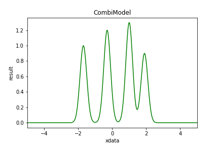
| Figure 6 shows example of a Combi Model. |
See also the combifit example.
KernelModels encapsulate kernel functions into a model. A kernel function is a an even integrable function. It is bound if the function value is 0 everywhere except for a region around zero.
km1 = KernelModel()                     # default: Biweight
km2 = KernelModel( kernel=Cosine() )
km3 = KernelModel( kernel=Tophat( 0 ) )
km4 = KernelModel( kernel=Tophat( 1 ) )
km5 = KernelModel( kernel=Tophat( 4 ) )
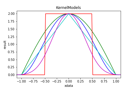
| Figure 7 shows examples of KernelModels. The Biweight kernel is in blue; the Cosine in green. The remaining 3 are 0, 1 and 4 convolutions of Tophat. |
SincModel is actually defined as a KernelModel with a Sinc kernel. Both GaussModel and LorentzModel could be defined in the same way, but are not.
Two dimensional kernel models also exist: Kernel2dModel. They come is 3 varieties: circular, elliptic and rotated.
km6 = Kernel2dModel( kernel=Gauss )
km7 = Kernel2dModel( kernel=Gauss, shape='elliptic' )
km8 = kernel2dModel( kernel=Gauss, shape='Rotated' )
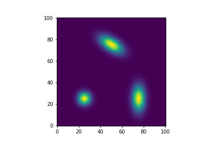
| Figure 8 shows examples of Kernel2dModels. Lower left is a circular 2d kernel; lower right an elliptic one and in the upper center a rotated one. |
Dynamic models can alter their behaviour by changing the number of parameters they contain. The purpose is to find the best model both in complexity (number of parameters) as in the parameter values itself. Fitters cannot do this, however the NestedSampler can.
Dynamic models have 2 extra methods grow() and shrink() that increase
cq. decrease the number of parameters. The rate of growth is governed by
a growPrior.
Dynamic models inherit from Model and from Dynamic.
mdl1 = PolynomialDynamicModel( 2 )
mdl2 = HarmonicDynamicModel( 0, maxOrder=6 )
mdl3 = RepeatingModel( 1, GaussModel(), minComp=1, maxComp=7,
    same=2, growPrior=JeffreysPrior() )
mdl1 starts as a polynomial of degree 2. It has a minimum degree of 0 and no maximum. The growPrior is an ExponentialPrior.
mdl2 starts as a HarmonicModel of order 0 with a maximum at 6. The growPrior is a UniformPrior.
mdl3 consists of at least 1 repetition of a GaussModel, up to 6 repetions are possible, where all GaussModels have the same value for the 2nd parameters (width).
Modifiable models can alter the internal structure of the model. E.g. the location of the knots in SplinesNodel. Again the purpose is to find the best internal structure and the best parameters that go with it. This can be done with NestedSampler
Modifiable models implement an extra method vary() that varies the
structure.
Most modifiable models are dynamic. They always inherit from Modifiable too.
It is indeed debatable whether the internal structure is not just another set of parameters. We chose this way as changes in the internal structure can be much more complicated than a simple change in value.
Some models are easier defined when it results in 2 (or more) values per
observation. Eg. the outcome of football match (3-1), or the position of
a star in orbit around another (distance and angle). These model have an
extra attribute ndout indicating how many output values per
observation are present.
The use of MultipleOutputProblem is needed in NestedSampler to flatten the multiple outputs.
The class AstropyModel is a wrapper for models originating from astropy.modeling.Model. Any FittableModel, wrapped in an AstropyModel can be used in BayesicFittings fitters and samplers.
from astropy import modeling
gm = modeling.models.Gaussian1D()
model = AstropyModel( gm )
Using UserModel, externally generated functionals of the form f(x:p) can participate.
def f( x, p ) :
    return p[0] * numpy.sin( p[1] * x + p[2] * numpy.log( x + p[3] ) )
model = UserModel( 4, f )       # 4 is the number of parameters
Optionally the partial derivatives df/dp and df/dx, and a name can be provided too. Otherwise numerically calculated values will be used.
model = UserModel( 4, f, userPartial=dfdp, userDeriv=dfdx,
                   userName="myName" )
Where dfdp and dfdx are methods: dfdp( x, p ) and dfdx( x, p ). The correctness of the (partial) derivatives can be checked with the method
model.testPartial( x, p, silent=False )
The methods are compared with numeric calculations of df/dp and df/dx.
A Fitter is an algorithm that minimizes the errors ε, the differences between the data, y, and the model, f(x:p).

The best fit is found through optimization of the parameters p. Traditionally this is done by finding the minimum of χ2, the sum of the squared errors. This least-squares method is computationally simple, especially if f is a linear function in its parameters p. These problems can be solved by (the equivalent of) one matrix inversion. Non-linear least-squares methods also exist. They are more demanding and require iterative methods to arrive at the minimum.
Other methods focus around the likelihood, which is maximized. Maximum likelihood is attained when the errors are minimal. Several likelihood functions are available in BayesicFitting. They are called ErrorDistribution. Using the GaussErrorDistribution is equivalent to using the least-squares method.
In a fitting process, it often occurs that data points are of different quality due to a variety of reasons. We can express the quatilies as either importance weights attached to the data points, or as a scale factor in the residuals. In our paper Kester and Mueller (2021) we expressed our preference for weights. However, we reconsidered it in the light of correlated errors in both axes. Kester 2023 Since version 3.1.0 of BayesicFitting, we offer both options.
Up on fitting, weights can be provided as a vector of the same length as
the data vector.
The behaviour of the fitter is such
that when a point has a weight of n, this is equivalent to a case where that
particular point is present in the dataset n times. This concept is
extended to non-integral values of the weights.
Weights could be derived from the standard deviations in a previous
calculation. In that case the weights should be set to the inverse
squares of the stdevs. However weights do not need to be inverse
variances; they could be derived in any other way. One specially usefull
feature of the use of weights, is that some weights might be set to zero,
causing those points not to contribute at all to the fit.
The accuracy is a (set of) numbers that represent a user provided estimate
of the size of the errors.
Accuracies do not change the "number of observations", as weights do. Each
measurement might have a different accuracy; it is still one measurement.
When choosing weight = accuracy-2, the difference only matters
in the calculation of the evidence.
Accuracy can be 1 number, valid for all data, or a vector of N, one value for
each data point. When there are possibly errors in both the dependent variable
and the independent variable, it can be a matrix of (N,2) or of (N,3).
In the latter case the third number is the (Pearson) correlation coefficient
between both variables.
As with Models there are two kinds of Fitters, linear an non-linear ones for linear and non-linear Models resp.
The landscape for linear models is monomodal i.e. it has only one (global) minimum. The linear fitter has generally no problem finding this minimum in one direct matrix conversion. It is fast and efficient. This package has 2 linear fitters: Fitter and QRFitter.
xdata = numpy.asarray( [1.0, 1.3, 1.5, 1.8, 2.0] )
ydata = numpy.asarray( [3.2, 3.9, 3.7, 4.0, 5.6] )
model = PolynomialModel( 1 )        # suppose liner relation
ftr = Fitter( xdata, model )        # define the fitter
par = ftr.fit( ydata, plot=True )   # optimal values for parameters
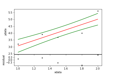
| Figure 9. A simple linear fit. The black dots are the data, the red line is the model and the green line a one-sigma confidence region. |
For non-linear models the χ2-landscape can be complicated. It can have many minima of which only one is the deepest. That is the one the fitter should find. Non linear fitters search for a gradient in the landscape to descend into the valley. Wherever a minimum is found, most fitters get stuck. There are several strategies to search the landscape but all of them are iterative. There is no single best strategy. It depends on the problem and on knowledge of the starting values for the parameters. This package has a dozen non-linear fitters.
Some non-linear fitters are strictly least-squares, others can be used as maximum likelihood fitters too.
xdata = numpy.asarray( [ 0.0, 1.0, 1.3, 1.5, 1.8, 2.0, 3.0] )
ydata = numpy.asarray( [-1.2,-0.9,-0.3, 0.0, 0.5, 1.0, 0.8] )
wgts  = numpy.asarray( [ 0.5, 2.1, 0.9, 1.3, 1.2, 0.8, 1.1] )  # weights
model = ArctanModel( )
ftr = LevenbergMarquardtFitter( xdata, model )  # define the fitter
par = ftr.fit( ydata, weights=wgts )            # optimal parameters
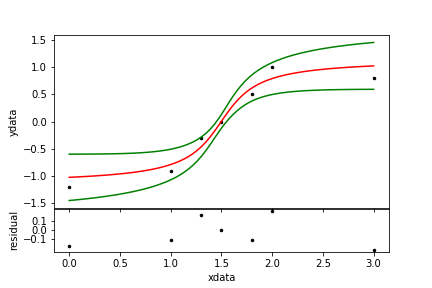
| Figure 10. A non-linear fit. |
LevenbergMarquardtFitter and CurveFitter are strictly least squares fitters. Other non-linear fitters like AmoebaFitter and the ScipyFitters can also be used as MaxLikelihoodFitters. The maximize the likelihood selected for the fitter.
ftr = AmoebaFitter( xdata, model, errdis='laplace' )
See the summerdays example.
When an optimal solution for the parameters has been found, a number of methods, all inherited from BaseFitter, are available to calculate standard deviations, noise scale, χ2, confidence regions and the evidence.
par   = ftr.parameters           # optimal parameters (same as above)
stdev = ftr.stdevs               # standard deviations on parameters
covar = ftr.covariance           # covariance matrix
chisq = ftr.chisq                # chisq at the optimal params
scale = ftr.scale                # scale of the remaining noise
yfit = ftr.getResult()           # fitted model values
yfit = model( xdata )            # same as previous
yband = ftr.monteCarloError()    # 1-sigma confidence region
All items above are more or less derived from the covariance matrix at the optimal parameter location.
The evidence is a number that indicates how probable a model is given the data. Evidence is not an absolute number; it must always be used to compare one model with other model(s).
For the casual user the evidence is the single item that lifts Bayesian fitting way above ordinary fitting. Wonderful things can be done with it that are beyond the standard ways. See my papers Kester (1999), Kester, Beitema and Lutz (2009), Kester and Bontekoe(2010), Kester (2010), Kester, Avruch and Teyssier (2014) and Kester, Higgins and Teyssier (2017).
The evidence can only be calculated when the limits on the parameters are provided. And, when the noise scale is fitted too, also for the scale. Priors for the parameters are assumed to be Uniform, for the scale it is JeffreysPrior.
It is up to the user to make sure that the optimal parameters and noise scale are well within the limits provided. Otherwise the gaussian evidence calculation is invalid.
limits = [-100.0,100.0]             # either 2 floats: all pars same limit. Or
lo = [-100.0, 0.0, 10.0]            # lower limits for the parameters
hi = [+100.0, 100.0, 20.0]          # upper limits for the parameters
limits = [lo,hi]                    # or 2 lists of floats
noiselim = [0.01, 10]               # limits on noisescale; all > 0
                                    # the 10-log evidence is obtained as:
evidence = ftr.getEvidence( limits=limits, noiseLimits=noiselim )
When in the above examples model has more than 3 parameters, the last limit
is repeated for all remaining cases.
There is a lot of mumbo-jumbo about priors. Formally, it is a representation of the knowledge about the problem before the data is taken into account. In abstracto one could imagine that there is no prior knowledge. In such cases the determination of priors seems highly subjective. However, in real life problems there are always limits on what can be measured in sensitivity, spectral range, duration, location etc. And consequentially on what values the parameters can attain.
See example on model comparison or harmonicfit for demonstration of the use of evidence to determine the best model. For instructions on when to optimize the noise scale too, see noise2 example. For a demonstration on the influence of noise on model selection see noise1 example.
The Fitters have the option to keep one or more parameters fixed during the fitting proces. It can be done in the construction of the fitter
fitter = SomeFitter( xdata, model, keep={key:value} )
to fix the parameter for the lifetime of the fitter. Or in the fit method itself.
params = fitter.fit( ydata, keep={key:value} )
to fix the parameter for this fit only. In both cases, key is a parameter index and value is a float at which the parameter should be fixed.
Note that fixing the parameter in the model replaces a parameter permanently with the chosen value.
See the fix parameters example for the suble differences between fixing the model, the fitter or the fit..
Sometimes the independent input xdata has more than 1 dimension. Then
a 2 or more dimensional models is required for a fit. The input,
xdata, is of the form array[N,D], where D is the number of dimensions
and N is the number of D-dimensional points. If N = 1 it can collapse to
array[D].
When the data to be fitted has the form of a map, or a cube, the xdata
still need to be an enumeration of all pixels. ImageAssistant
extracts the necessary xdata from the map, and converts the map values
in 1-d ydata. It is silently invoked by the fitter when the keyword
map is set.
y = numpy.zeroes( (3,4), dtype=float )  # some empty map
mdl = PolySurfaceModel( 0, 0 )
fitter = Fitter( y, mdl, map=True )     # use y here as xdata
print( fitter.xdata.shape )             # show shape of internal xdata
> [12,2]
pars = fitter.fit( y )                  # use y here too, now as ydata
print( fitter.yfit.shape )              # show the shape of the result
> [3,4]                                 # same as the original map y
print( mdl( fitter.xdata ).shape )      # the model however, returns
> [12]                                  # a 1-d version of y
See simplemap for more about the use of the keyword "map". And randommap for random observation in a 2-d object and about the explicit use of ImageAssistant.
A special fitter is RobustShell. It is a shell around any other fitter. RobustShell iteratively de-weights outlying points. It makes the fit more robust in the presence of a minority of outliers i.e. points that should not partake in the fit. The de-weighting process is governed by one of the kernels.
np = 101                                #
xdata = numpy.linspace( 0, 1, np )      # make 101 datapoints
ydata = numpy.linspace( 0.3, 0.5, np ) + 0.3 * numpy.random.rand( np )
no = 20                                 # 20 outliers
out = numpy.asarray( np * numpy.random.rand( no ), dtype=int )
val = 1 * numpy.random.rand( no )
ydata[out] += val                       # at random place, value
pm = PolynomialModel( 1 )
ftr = Fitter( xdata, pm )
par0 = ftr.fit( ydata )                 # simple fit
rft = RobustShell( ftr )
par1 = rft.fit( ydata )                 # robust fit
rwgt = rft.weights                      # resulting robust weights
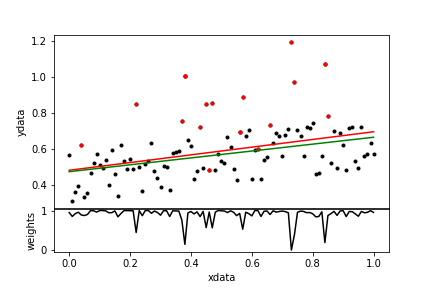
| Figure 11. A robust fit. The data points are in black; the outliers are red. The normal fit is the red line; the robust fit is green. In the lower panel the resulting weights are displayed. |
Robust fitting is even more dangerous than ordinary fitting. Never trust the results without thorough checking.
This more elaborate example shows the suppression of irrelevant points.
NestedSampler is a novel technique to do Bayesian calculations. It samples the Posterior while integrating it to calculate the evidence. The evidence and the samples from the posterior are the main results of NestedSampler. From the samples, the optimal values for the model parameters, its standard deviations etc can be calculated.
Nested sampling is an idea of David McKay and John Skilling. Skilling has written a separate chapter in Sivia's book explaining the Nested Sampling idea, including an algorithm in C, which served as the basis (via JAVA) for our implementation.
NestedSampler applies an ensemble of walkers, initially evenly distributed over the prior probability. Then an iterative process is started. Every iteration the walker with the lowest likelihood is discarded and replaced by a copy of one of the remaining walkers. The copied walker is wandered around randomly by one or more Engines, provided it keeps a higher likelihood than the value of the discarded walker. This way the ensemble of walkers stays randomly distributed over the prior while the ensemble as a whole slowly ascends the likelihood to the top. The discarded walker is kept as a sample of the posterior, appropriately weighted. NestedSampler uses Priors for the initial distribution of the parameters and an ErrorDistribution to calculate the likelihoods.
PhantomSampler is an extension of NestedSampler, in the sense
that it uses (some of) the intermediate positions that the walkers take
when they are wandered around by the Engines. These positions are
commonly known as Phantoms. How many phantoms are used, is governed by
the keyword step=. In each iteration step percent of the ensemble is
replace by new phantom walkers. The benefits of the scheme is a step-fold
increase in calculation speed; the downside is less precision and less
exploratory power. The value of step is limited to 10.
NestedSampler needs more information to run than ordinary Fitters. It needs priors for all its parameters and it needs a likelihood function.
We start off defining some data.
xdata = [1.0, 2.0, 3.0, 4.0, 5.0]
ydata = [0.2, 1.3, 4.5, 1.4, 0.1]
Set up the model with limits on the uniform priors of the parameters.
model = GaussModel()
lolim = [-10.0, 0.0, 0.0]           # low limits on the params
hilim = [+10.0, 5.0, 5.0]           # high limits
model.setLimits( lolim, hilim )     # use UniformPrior with limits
The likelihood is calculated by the GaussErrorDistribution. By default it has a fixed scale. However in most real cases ( see noise2 example ) it is better to treat the scale as a hyperparameter, which needs a prior, by default a JeffreysPrior, and limits.
limits = [0.01, 10]
ns = NestedSampler( xdata, model, ydata, limits=limits )
We execute the program as
logE = ns.sample()
where logE is the 10log of the evidence.
After the call to sample() optimal parameters, standard deviations, scale and the
optimal fit of the model are available from NestedSampler.
param = ns.parameters
stdev = ns.standardDeviations
scale = ns.scale
yfit  = ns.modelfit
The values are actually obtained from the SampleList, a list of Samples, that is the other result of the NestedSampler. From the SampleList numerous items can be extracted.
slist = ns.samples
param = slist.parameters        ## same as params above
mlpar = slist.maxLikelihoodParameters
In the examples directory the use of NestedSampler is demonstrated in HD2039 and outliers2.
NestedSolver applies the same algorithm to OrderProblems, where the problem is solved by finding an optimal order. The parameters are no floats but integers, that provide an ordering of the data. The iconic example is the traveling salesman problem. However all kind of scheduling problems fall in this category too.
A problem specific cost function functions as a (unnormalized) likelihood.
The NestedSolver returns the last (best) sample as the solution to the order problem.
The Problem classes have been introduced in version 2.0. They are meant to broaden the applicability of NestedSampler beyond the classic problems that we addressed before. A Problem collects all items that are needed to solve the problem, where the parameters constitute the solution.
A ClassicProblem consists of a parameterized model with a list of measured data at the locations of the indepemdent variables. Optionally there are weights and/or accuracies. The ClassicProblem is invoked by default.
Other Problems need to be separately invoked.
In case there could be errors both in the independent variable (x) and in the dependent variable (y), the ErrorsInXandYProblem should be invoked. To solve this kind of problems we need to assign extra parameters for all values of the independent variable (x). These new positions need to be estimated along with the parameters of the model itself. These new parameters need a prior. A GaussPrior with a fixed scale is advised. The priors will be centered on the measured x values.
prior = GaussPrior( scale=0.1 )
problem = ErrorsInXandYProblem( model, xdata, ydata, prior=prior )
ns = NestedSampler( problem=problem )
evidence = ns.sample()
The extra parameters needed here, are called nuisance parameters.
For models that naturally produce 2 or more dimensional outputs (like the StellarOrbitModel) the MultipleOutputProblem need to be invoked. It just reshapes the residuals into a 1-dim array before it is used to calculate the likelihood..
The EvidenceProblem uses the evidence calculated for different instantiations of a Modifiable model, as "likelihood" in a next level of Bayes' rule to determine which of the instantiations is best. The "likelihood" to be used here is the ModelDistribution. It calculates the evidence of the model either as a Gaussian approximation or by using NestedSampler on a ClassicProblem.
The OrderProblem is for integer valued problems where the solution is found in some ordering of the data. The only example now is the SalesmanProblem.
See below for lists of available Problems. More Problems can be expected in later versions.
A Sample is a collection of items.
Samples can be collected in a SampleList. The resulting samples from the posterior are collected in a SampleList.
When using the samples of the posterior for other purposes than are provided in SampleList, all items derived from individual Samples should be weighted with
weight = exp( sample.logW )
before averaging them.
The internal ensemble of trial points is designed as a WalkerList, or a list of Walkers. Walkers are similar to Samples, except that they have a Problem in stead of a Model.
The number of walkers can be set with the ensemble keyword. By default
ensemble=100. The number of walkers that are discarded in every
iteration can be set with discard. By default discard=1. When
discard is greater than 1, it might be profitable to set the keyword
threads=True to randomize each walker in a separate thread. And
finally the keyword maxsize can be used to limit the amount of
resulting samples. When the size of the sample list is larger than
maxsize, the samples with the smallest weights are thrown out. By
default maxsize=None.
ns = NestedSampler( xdata, model, ydata, ensemble=200, discard=5,
                    threads=True, maxsize=5000 )
Before NestedSampler can be started with ns.sample() the Model
should be provided with Priors for all parameters. The same holds
for the ErrorDistribution if it has unknown hyperparameters.
Priors are attributes of the simple model.
gm = GaussModel()
amppr = ExponentialPrior( scale=10 )        # prior on amplitude (>0)
cenpr = UniformPrior( limits=[-1,1] )       # prior on center
widpr = JeffreysPrior( limits=[0.1, 2] )    # prior on width
gm.priors = [amppr, centpr, widpr]          # set the priors
The default prior for model parameters is the UniformPrior. The UniformPrior needs limits: low and high. When a Model is provided with limits it sets the priors as UniformPrior with the limits.
low = [0.0, 2.0, -10]           # lower limits
high = [10, 10, 10]             # upper limits; high[k]>low[k] forall k
model.setLimits( low, high )    # makes list of 3 uniformPriors with limits
When the model has more parameters than the length of the limits cq. priors, the last one is repeated for all remaining parameters.
The priors are attributes of the simple models. In compound models the priors are taken from the constituent simple models, including the repetition of the last prior. So priors should be set, before using the simple model in a compound one.
Suitable Priors can have limits, which may be circularly folded for parameters that represent a phase or a period. The circular keyword either takes a boolean, to indicate that it is circular between the limits, or a float to define the period of circularity.
lp = LaplacePrior( center=1.0, scale=0.5, circular=3 )
pr = UniformPrior( limits=[2,3], circular=True )
See below for lists of available Priors.
The ErrorDistribution determines the likelihood function.
Except the PoissonErrorDistribution and the BernoulliErrorDistribution all others have one or more HyperParameters which are governed by a Prior, unless they are known in advance.
dis = GaussErrorDistribution( )
dis.setLimits( [0.1, 1.0] )
ns = NestedSampler( xdata, model, ydata, distribution=dis )
The GaussErrorDistribution is an descendant of the abstract ScaledErrorDistribution. As is the LaplaceErrorDistribution, the ExponentialErrorDistribution and the UniformErrorDistribution. They are all different norms of the residuals. The ExponentialErrorDistribution has another HyperParameter called power, It is the (fractional) norm.
The PoissonErrorDistribution is for counting experiments, with integer-valued data.
The BernoulliErrorDistribution is for categorical data. It needs a
model with as much outputs (ndout) as there are categories. The
dependent variable (y) contains an integer (< ndout) indicating to which
category this data point belongs. Each model output gives the
probability (0 <= p <= 1), that the item falls in that category.
At present only the SoftMaxModel is available.
The use of a mixture of 2 error distributions (MixedErrorDistribution) is shown in outliers2.
To avoid certain combinations of parameters a "constrain" attribute can be attached to an ErrorDistribution. It needs to be a user-provided callable method in the form
def insideSphere( logL, problem, allpars, lowLogL ) :
    return logL if numpy.sum( numpy.square( allpars ) ) < 1.0 else lowlogL - 1

errdis.constrain = insideSphere
When the to be avoided condition occurs logL is returned as one less than the low likelihood limit so it will never be selected. Otherwise logL should be returned unchanged. It should be noted that the acceptable area should be large enough that it can reasonly be sampled randomly for an initial ensemble of Walkers.
See below for lists of available ErrorDistributions.
Since version 2.0 the ErrorDistributions has changed its interface.
Previously it was called as GaussErrorDistribution( xdata, ydata ).
Now the responsiblities of ErrorDistribution and Problem are better separated.
For the only OrderProblem at present we provide the DistanceCostFunction to obtain a simile of the likelihood.
An Engine is piece of programming that moves a walker around in parameter space such that the resulting walker is distributed randomly over the priors within the constraint that the likelihood associated with the walker remains higher than a preselected level.
The engines of choice for continuous parameter estimation are the GalileanEngine and the ChordEngine.
The GalileanEngine starts at the copied walker. It selects a random step in parameter space and moves forward half a dozen times. When a step trespasses the likelihood boundary it mirrors on the boundary to get back into allowed space. If that is also unsuccesfull in reverses its steps.
The ChordEngine selects a random direction, though its starting point. It extends that direction until is is outside the the selected level. It selects a random point on the line. If it is inside the level, it is the new point. Otherwise replace one of the endpoints and select again.
The initial distribution of the walkers is made by StartEngine.
When the model is dynamic, the BirthEngine and DeathEngine are added to the engine list to govern the increase and decrease of the number of parameters.
When a model is modifiable, the StructurEngine is added to the engine list, to randomly change the structure of the model.
For the SalesmanProblem 5 engines are provided that all change the order in the parameters by some way: MoveEngine, ReverseEngine, SwitchEngine, LoopEngine, ShuffleEngine and NearEngine.
Engines are selectable in the construction.
The keyword rate governs the speed of the engines. High rate equals
high speed equals low accuracy.
ns = NestedSampler( xdata, model, ydata, rate=0.5,
                    engines=["galilean", "gibbs", "chord", "step"] )
See below for lists of available Engines.
Each iteration of NestedSampler the Engines in the list are selected in a random order and executed until enough movement is provided to the Walker. By setting the attributes "slow" to an Engine, it is selected only every slow-th iteration. With
ns.engine[1].slow = 3
the GibbsEngine is selected every third iteration only. To be used for expensive, biased or unbalanced Engines.
Just like the Fitters NestedSampler can have a keywords
weights to set weights and keep to keep some parameters fixed at a
known value. Both keywords act as in the Fitters.
Also analog to the fitters, the sample() method can have the
keywords keep and plot.
The keyword verbose determines how much output the program generates.
The keyword seed seeds the random number generator, to ensure the same
random sequence each run.
ns = NestedSampler( xdata, model, ydata, weights=wgts, keep={0:1.0},
                    seed=123456, verbose=2 )
logE = ns.sample( keep={2:3.14}, plot=True )
All classes are listed with a one-line purpose. They are organized by their functionality into 5 sections, models, fitters, nested sampling, kernels and miscellaneous.
Dynamic models have an adaptable number of parameters. They can only be used with NestedSampler.
Base Models should never be called directly. They contain features common to all classes that inherit from them.
minimize, to fit
data to a model.
ScipyFitter contains the classes:
BaseFitters contain common methods for fitters that inherit from them.
Kernels are even functions that are integrable over (-inf,+inf). A kernel is bound when it is zero outside (-1,+1)
They can be encapsulated in a KernelModel or in a 2dim Kernel2dModel. They also find use in the RobustShell.
| name | function | bound | comment |
|---|---|---|---|
| Biweight | ( 1-x2 )2 | true | |
| CosSquare | cos2( 0.5 π x ) | true | |
| Cosine | cos( 0.5 π x ) | true | |
| Gauss | exp( -0.5 x2 ) | false | |
| Huber | min( 1, 1/|x| ) | false | improper because infinite integral |
| Lorentz | 1 / ( 1 + x2 ) | false | |
| Parabola | 1 - x2 | true | |
| Sinc | sin(x) / x | false | do not use in RobustShell |
| Tophat | convolution | true | 0 to 6 convolutions of Uniform |
| Triangle | 1 - |x| | true | |
| Tricube | ( 1 - |x|3 )3 | true | |
| Triweight | ( 1 - x2 )3 | true | |
| Uniform | 1.0 | true |