The behaviour of splines of different orders is explained in the table.
| order | behaviour between knots | continuity at knots |
|---|---|---|
| 0 | piecewise constant | not continuous at all |
| 1 | piecewise linear | lines are continuous (connected) |
| 2 | parabolic pieces | 1st derivatives are also continuous |
| 3 | cubic pieces | 2nd derivatives are also continuous |
| n>3 | n-th order polynomials | (n-1)-th derivatives are also continuous |
From here on we work with cubic splines on a random grid unless otherwise indicated. It is quite easy to extend the ideas to lower or higher orders.
Assume we have a set of knots as in
  |------------|------|---------|-------------------|---
  k0           k1     k2        k3                  k4   etc..
The set of knots defines the domain where the spline model is valid.
We define a 3rd order polynomial to the first knot segement (k0,k1).
| f0(x) = p0 + p1 x0 + p2 x02 + p3 x03 |
For the second segment (k1,k2) we extend the function of the previous segment and add
| f1(x) = | p4 x13 | if x > k1 |
| 0 | if x < k1 |
Note that the function f1 is continuously differentiable to the 3rd derivative. For x < k1 it is all 0; for x > k1 it is a 3rd order polynomial and at x = k1 the derivatives from the up-side are all 0, equal to those from the low-side.
For the next segments we repeat this procedure.
So in the end we have a spline function f(x) as
| f(x) = | p0 + p1 x0 + p2 x02 + p3 x03 + ∑ pi+4 xi3 |
This simple algorithm has two disadvantages. Firstly it is not symmetric. We could also have started at the end of the domain and worked our way to the beginning. We would obtain a different spline representation, not better or worse than the first. Secondly the parameters are not localized. Each parameter influences the result over the complete domain. Preferably one parameters affects only one part of the model without influencing the others. In this algorithm a parameter affects all later parameters.
Even with these defects it is a usefull and fast algorithm. The algorithm is implemented in SplinesModel.py.
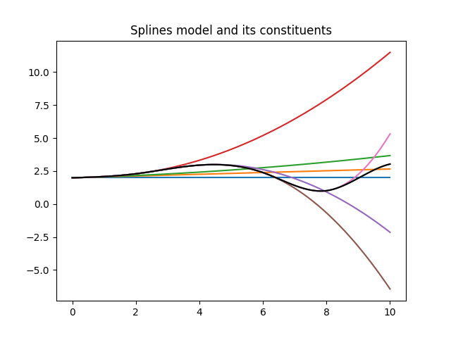
In figure 1 the model is displayed with all its components.

| Figure 1 shows the the splines model and all its components. The knots are located at [0,2,4,6,8,10]. |
Figure 1 is made with the following piece of python code.
  from BayesicFitting import SplinesModel
  import matplotlib.pyplot as plt

  x = numpy.linspace( 0, 10, 101, dtype=float )
  kn = numpy.linspace( 0, 10, 6, dtype=float )
  sm = SplinesModel( knots=kn )

  par = [1.989, 0.066, 0.010, 0.016, -0.046, -0.028, 0.210, -0.286]
  sm.parameters = par

  part = sm.partial( x, par )
  yf = numpy.zeros( 101, dtype=float )
  for k in range( sm.npars ) :
      yf += part[:,k] * par[k]
      plt.plot( x, yf )

  plt.plot( x, sm.result( x, par ), 'k-' )
  plt.title( "Splines model and its constituents" )
  plt.show()
Carl de Boor (in "A Practical Guide to Splines.", (1978) Springer-Verlag. ISBN 978-3-540-90356-7.) designed a recursive algorithm where each recursion produces a set of base splines of a higher order.
John Foster and Juha Jeronen implemented de Boor's algorithm in Python in the bspline package. We encapsulated the bspline package into our BSplinesModel.py.
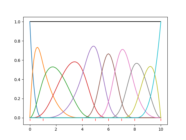
In figure 2 a set of basis splines of order 3 is displayed, using parameters all equal to 1.0. The knots are at [0,1,4,5,6,7,8,10]; 8 knots resulting in 10 basis functions and as many parameters. The sum of the components is the black line constant at 1.0.

| Figure 2 shows the de Boor splines model and all its components. The position of the knots is indicated with red bars low in the plot. |
Unfortunately the recursive implementation in BsplinesModel is about 20 times slower than the the splines in SplinesModel.
We have a 3rd order polynomial between the first 2 knots.
f(x) = a + b x + c x2 + d x3
          f1
    |------------|----
    x0           x1
The property 3-smooth implies that the function and it first and
second derivative are 0 at x1, while the function is unbound,
arbitrary at x0. We normalize the blob in x0 at 1.
f1(x1) = 0
f1'(x1) = 0
f1"(x1) = 0
f1(x0) = 1
Now we have 4 equations with 4 unknown coefficients (a,b,c,d) which we can solve.
         f1          f2
    |------------|------|---
    x0           x1     x2
f1(x) = a1 + b1 x + c1 x2 + d1 x3
f2(x) = a2 + b2 x + c2 x2 + d2 x3
The function, f1 is 1-smooth at x0. f1 and f2 are 3-smooth at x1 and f2 is 3-smooth with 0 at x2. Again we need a normalization at x1.
f1(x0) = 0
f1(x1) - f2(x1) = 0
f1'(x1) - f2'(x1) = 0
f1"(x1) - f2"(x1) = 0
f2(x1) = 0
f2'(x1) = 0
f2"(x1) = 0
f1(x1) = 1
We have 8 equations and 8 coefficients (4 per function) so it can be solved directly.
| blob | x0 | x1 |
|---|---|---|
| 1 | 0-smooth | 3-smooth |
| 2 | 1-smooth | 2-smooth |
| 3 | 2-smooth | 1-smooth |
| 4 | 3-smooth | 0-smooth |
In case we have a cubic spline on a set of 3 knots, x0 .. x12, the smoothnes at the knots is given in the table below.
| blob | x0 | x1 | x2 |
|---|---|---|---|
| 1 | 0-smooth | 3-smooth | n/a |
| 2 | 1-smooth | 3-smooth | 3-smooth |
| 3 | 2-smooth | 3-smooth | 2-smooth |
| 4 | 3-smooth | 3-smooth | 1-smooth |
| 5 | n/a | 3-smooth | 0-smooth |
S(x:p) = ∑ pk fk( x )
S(x:p) = ∑ pk ( ak + bk x + ck x2 + dk x3 )
S(x:p) = ∑ ( pk ak ) + ∑ ( pk bk ) x + ∑ ( pk ck ) x2 + ∑ ( pk dk ) x3
The coefficients and the parameters can be multiplied together, forming
one piecewise 3-order polynomial function of the x's.
This algorithm proved to be 10 times faster than the recursive one.
Still slower by a factor 2 than the first one.
The advantages we obtained though, are that the blobs are independent.
when one parameter changed only localized effects are seen. Even when
the position of a knot shifts, adjacent knots are only slightly
affected. This opens the option of a DynamicBasicSplinesModel.