Here we present some examples of what the BayesicFitting package is capable of.
Clicking on one of the images will display the code which produced the fit and ultimately the image. Originally the code is in the form of a jupyter notebook. Here it is converted to html.
It is allowed, even encouraged to copy and paste the code lines and adapt them to other problems.
More examples in the original jupyter notebook, can be found on github.
|
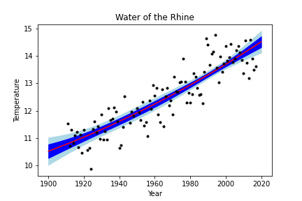
The temperature of the Rhine water is measured since 1911 at Lobith, where it enters the Netherlands. It seems to have a slight curvature, so we fit it with a 2nd order polynomial. The model is shown in red; the confidence region is in blue. | |
|
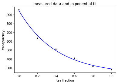
Julius had to do an experiment for his chemistry class. He needed to measure the transparancy of a glass of water mixed with increasing amounts of strong tea. For the measurements he used an app on his phone. As a light source he had a desk lamp. | |
|
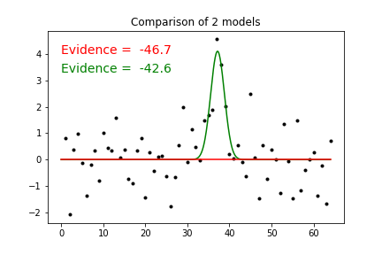
We show spectral line data in 64 frequency channels from a radio astronomy spectrometer. The data fitted with 2 models. A constant model assuming there is no spectral feature in the data, shown in red. And a gaussian model, assuming a spectral feature around channel 40, shown in green. The green model is more probable than the red one by 103.9 : 1. | |
|
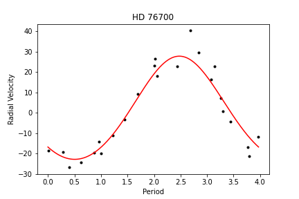
The star HD 76700 has at least one planet cycling around it, giving rise to slight variations in the radial velocity. These radial velocity data are analysed to find out the orbital elements of the exoplanet. | |
|
The star 83 Aquarii is a visual double star, that orbit each other in about 25 years. Over 100 years of data are analysed to abtain the orbital elements. In the picture above we see the orbit of 83 Aqr as it appears on the sky. (North down, east left). The black ellipse is the projected orbit of the secundary star. It is moving anti-clockwise. The observations at the colored points are connected to the orbit location at the same time. The lines represent the misfits. The colors indicate when they are taken: blue < 1950; 1950 < red < 2000 and green > 2000. The main star is located at (0,0) where the back * is plotted. Through it in magenta is the line of nodes, i.e. where the sky through the main star crosses the orbit. On one side the ascending node, the place where the orbiting star crosses the sky plane and is moving toward us. At the other side, at the descending node, the orbiting star crosses the sky plane away from us. The black line from the main star to the orbit indicate the location of the periastron, the place where the stars as closest together. |
